flowchart TD
    A[Were the comparisons planned in advance?] -->|Yes| B[Pairwise comparisons only?]
    A -->|No| C[Pairwise comparisons only?]
    B -->|Yes| D["If all C = a(a-1)/2 comparisons, then use Tukey"]
    B -->|Yes, alternative route| E["Compare critical values: Tukey vs Bonferroni, based on df and C"]
    B -->|No, includes complex comparisons| F["Compare critical values: Scheffe vs Bonferroni, based on df and C"]
    C -->|Yes| G[Use Tukey]
    C -->|No, includes complex comparisons| H[Use Scheffe]
Type I Error Correction: Multiple Comparison Procedures
Introduction
In the previous lesson, we covered how to formulate and test contrasts after a significant omnibus ANOVA. But we left something important unaddressed: what happens when you run many of those tests? Initially, this might not be seen as a concern, however this is a very important aspect of psychological research. Each test you run has a chance of producing a false positive, and the more tests you run, the more that risk compounds. If you carelessly start running a bunch of tests, you will eventually get a Type I error. This fact is inevitable and enescapable.
Think about it this way, imagine standing in front of a mirror and inspecting yourself for flaws. Even if you are a perfectly healthy and beautiful human being, the longer and more carefully you look, the more likely you are to notice something like a blemish, an asymmetry, or a hair out of place. None of these might mean anything, but the sheer act of repeated searching guarantees you will eventually land on something that looks wrong, and this will cause your self esteem to plummet, even if the “flaw” was never a big deal! The more you are looking for personal flaws, the more you are going to find one regardless of how insignificant they are.
Type I error inflation works the same way. Each additional significance test is another pass in the mirror, and the more passes you take, the more likely you are to flag something as a “real” finding purely by chance.
This lesson is about how to keep that risk of finding false results under control.
We will continue with the hypertension dataset from the previous lesson, but it is labeled MultipleCorrections.sav this time. This data consists of four treatment groups (drug therapy, biofeedback, dietary modification, and a combination treatment), with blood pressure as the dependent variable. The combination treatment group had the lowest mean (\(\bar{X} = 83\)), while the other three groups had means of 91.4, 93, and 92 respectively.
1. The Multiple Comparisons Problem
Why Running Many Tests Is Dangerous
When you reject the null hypothesis at the level \(\alpha = .05\), you are accepting a 5% chance that you are wrong and that the effect you found is a false positive. This is called a Type I error. That 5% is arbitrary, but it is generally the recommended manageable risk for a single test for psychology. In clinical settings, you might use \(\alpha = .01\) instead, but we will use .05 going forward.
We distinguish two kinds of error rates:
- Per-comparison error rate (\(\alpha_{PC}\)): the false positive rate for a single test, the one you set directly (e.g., .05).
- Experimentwise error rate (\(\alpha_{EW}\)): the probability of making at least one Type I error across the entire set of tests you are running.
The former is what you set directly by choosing your significance threshold before running a test. The latter is what researchers need to worry about as they publish their studies: it is the real probability that your study produced at least one false positive result.
A practical way to think about it is that \(\alpha_{PC}\) is the concern of a researcher evaluating a single isolated test, while \(\alpha_{EW}\) is the concern of a psychologist writing up a results section and asking whether their pattern of significant findings can be trusted. If you ran one contrast and it was significant, \(\alpha_{PC}\) is what matters. If you ran six contrasts and three of them were significant, \(\alpha_{EW}\) is what should haunt you.
For a set of contrasts, the experimentwise error rate is:
\[\alpha_{EW} = 1 - (1 - \alpha_{PC})^C\]
where \(C\) is the number of comparisons being made. With just 3 comparisons at \(\alpha = .05\):
\[\alpha_{EW} = 1 - (1 - .05)^3 = 1 - (.95)^3 \approx .143\]
So, if you did 3 tests, your real Type I error rate is actually 14%, not 5%. With 10 comparisons it climbs to about 40%. You are no longer doing science at \(\alpha = .05\). You are just conducting a lottery and hoping you get lucky.
Luckily, there are ways to help mitigate this issue that researchers need to be aware of. Unfortunately, most people don’t do this, since they either A) don’t know about these things or B) don’t want to lose their “significant” results (i.e., they don’t want to admit they might have had false findings).
It’s a bit disheartening the ammount of researchers who don’t even consider experimentwise error rates, but you, reader, can be the change we need!
Planned vs. Post Hoc Comparisons
An important distinction for choosing how to control Type I error is whether your mean comparisons were planned or post hoc.
A planned contrast is one you decided to test before looking at the data, based on your theoretical hypotheses. You committed to it in advance.
A post hoc contrast is one you decided to test after examining the data. For example, after noticing that two particular group means look far apart.
This distinction matters more than it might seem. Suppose you run a four-group study and after seeing the results you decide to test the largest-looking mean difference. It feels like you are only running one test. But in reality, you implicitly scanned all possible pairwise differences before choosing that one. The comparison that “caught your eye” is almost by definition the most extreme one in the data, which means it is also the one most likely to be a false positive. You did not really run one test. You ran all of them mentally and selected the winner.
This is called data-driven science and is generally frowned upon within psychology. This type of behavior has heavily contributed to replication issues, since researchers are just looking for any significance rather than actually doing hypothesis testing from theoretical decisions.
To account for these issues of post hoc testing, the number of comparisons you must account for is not just the ones you formally tested, but the entire family of comparisons that your selection process implicitly considered.
2. How to Correct for Experimentwise Error?
The solution to Type I error inflation is to apply a multiple comparison procedure, which is a method that adjusts how you evaluate significance when running more than one test. These procedures make sure your experimentwise error rate stays at .05 rather than ballooning beyond it. The general idea behind all of these methods is the same: make each individual test harder to pass, so that the cumulative probability of any false positive across all tests stays controlled.
For instance, instead of requiring \(p < .05\) to declare a contrast significant, you might require \(p < .017\) if you are running three tests. Each individual hurdle is higher, but the payoff is that your overall false positive risk across all three tests stays at .05.
There is no single universal correction, and each one differs in the situations they are designed for. The right choice depends on two things:
Whether your comparisons were planned before data collection or chosen post hoc after examining the results.
Whether your comparisons are pairwise only (one group compared to another group), or include complex comparisons that involve averages of multiple groups.
The three most common procedures are Bonferroni, Tukey, and Scheffé. We will cover each in turn, using the hypertension dataset to illustrate.
Before we go into detail, a handy decision tree below summarizes the recommendations depending on your scenario (Note, “CV” stands for critical value, which we will get into).
3. Bonferroni Correction
The Logic
Bonferroni is the simplest approach. If you are running \(C\) tests and want your overall experimentwise error rate to be \(\alpha_{EW} = .05\), you just divide your significance threshold by \(C\):
\[\alpha_{Bonferroni} = \frac{\alpha_{EW}}{C} = \frac{.05}{C}\]
Each individual comparison must then have \(p < \alpha_{Bonferroni}\) to be declared significant. Think of your total allowable false positive risk as a budget. You only have five cents to spend across all your tests. Bonferroni simply splits that budget evenly, giving each test an equal share. The more tests you run, the smaller each share gets, and the harder each individual test becomes to pass.
For example, if you plan 3 comparisons:
\[\alpha_{Bonferroni} = \frac{.05}{3} = .0167\]
In this case, the budget for individual tests was \(\alpha_{Bonferroni}=.0167\) each for your allowance of \(\alpha_{EW}=.05\).
This value of .0167 is conservative, meaning it is harder to reject individual tests.
Terminology note on testing: “Conservative” means tests are harder to reject. “Liberal” means tests are easier to reject. One is not better than the other inherently. It depends the context. With concern to Type I error, however, the more conservative your test, the least likely you are to make a false positive. However, this comes with a trade off in statistical power. So the more conservative your test is, the harder it is to reject. That means it is harder to make a false positive, but as a result, it also is harder to make a correct positive. Often times, when choosing your methods and anlyese, you will have to decide where on this trade off you want to be. But more on this later.
Bonferroni is a blunt instrument for correction, but it always works, as long as you can specify \(C\) in advance. Because of this, it is the most universally applied correction as it can be applied in any scenario. It just depends on what you set \(C\) as.
Setting C
Deciding what \(C\) should be is where researchers sometimes go wrong. The rule is: \(C\) must reflect the number of comparisons that were realistically considered, not just the ones you formally ran.
- If you planned a specific set of \(C\) comparisons before data collection, \(C\) is that number.
- If you want to test all pairwise comparisons (or if your original plan was all pairwise but you ended up testing fewer), \(C\) must be set to \(\frac{a(a-1)}{2}\), where \(a\) is the number of groups.
- If you intended to test a subset of pairwise comparisons but then tested additional ones after seeing the data, again \(C = \frac{a(a-1)}{2}\).
The key principle: if you let the data influence which comparisons you run, your \(C\) needs to expand to cover all comparisons that could have been selected. This controls for the “eyeballing it” scenario.
For an example, let’s say after running an ANOVA for a variable with 5 groups, you want to test a pairwise comparison. This means you would have seen the results and the sizes of the means, so it is appropriate to control for all possible pairwise comparisons. That means you set \(C\) as
\[C =\frac{5(5-1)}{2}=\frac{20}{2}=10\]
Therefore, your Bonferroni corrected alpha level is \(\alpha_{Bonferroni}=.05/10=.005\). This means for any of the pairwise comparisons you make as a contrast for this ANOVA, the p values must be less than .005 to be considered significant.
The Test Statistic and Critical Value
The F statistic and confidence interval formulas for Bonferroni contrasts are identical to those from the Contrasts lesson, nothing changes there. You can look those up if you want to. What does change is the critical value of your significance test. Under the Bonferroni correction with equal variances:
\[CV = F_{\alpha/C;\; 1,\; df_{error}}\]
This is more or less the same as what you would use for any contrast, except instead of just using \(\alpha = .05\), you use whatever \(\alpha/C\) comes out to be.
This new critical values redefines the confidence intervals as well. So as a result, the confidence intervals for Bonferroni corrected tests become wider.
Advantage and Limitation
The main advantage of Bonferroni is its simplicity and flexibility — it works for any set of contrasts, pairwise or complex, planned or post hoc (as long as \(C\) is finite and specifiable).
The limitation is power. As \(C\) grows, each individual threshold becomes more and more stringent, making it harder to detect real effects. For a small number of planned comparisons, Bonferroni is excellent. For a large number, or for post hoc complex comparisons where \(C\) is theoretically infinite, it breaks down.
Bonferroni in SPSS
There is no official way to do Bonferroni in SPSS. ALl you need to do is look at your p value in the output, and compare that to what your \(\alpha_{Bonefrroni} = \alpha/C\) level. However, if you want corrected confidence intervals, you need to manually set your confidence level
There’s different ways to do this in SPSS, however, I highly recommend using MANOVA because it gives you full control and scope over everything it is doing.
MANOVA pressure BY treat (1 4)
/print=cellinfo(means)
/error=within
/cinterval =individual(.9833) /* add this line to specific confidence levels
/contrast(treat) = special (1    1     1     1
                            1    1     1    -3
                            .5   .5   -.5  -.5
                            1   -1     0     0)
/design = treat(1) treat(2) treat(3).
The /cinterval line is where you specify the new Bonferroni confidence level. This level is simple equal to \(1-(\alpha/c)\), so in our example with 3 contrast comparisons, it is \(1−(.05/3)=1-.0166=.9833\). It is important to remember to put this in your syntax before you estimate the model or else you will get the wrong confidence intervals, and thus might be giving the wrong results.
The output for this would look like:
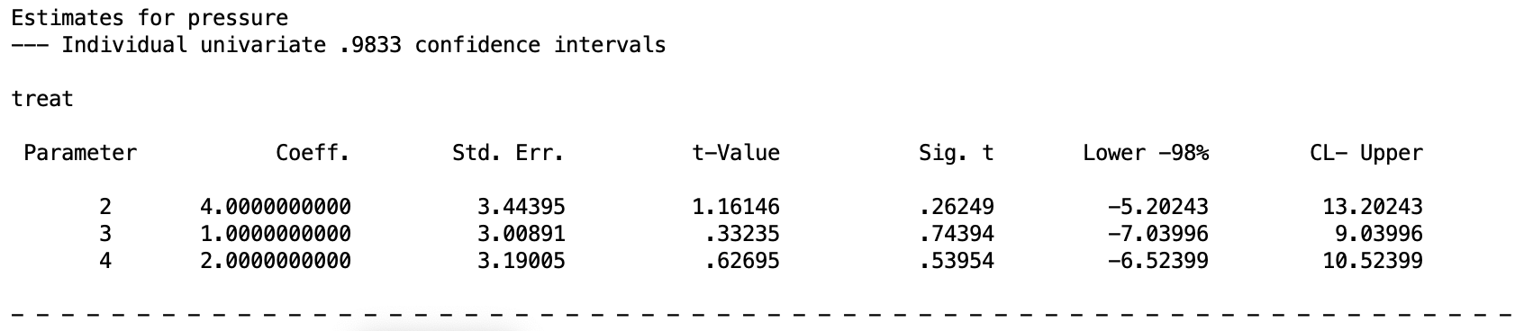
This piece of the output contains each of the contrasts I specified for treatment above. This isn’t the best example, but we can see that the p values are greater than \(\alpha/c = .0166\), thus none are significant after controlling for experimentwise error rate. The confidence intervals are also adjusted appropriately, as you can see in the top “.9833 confidence intervals”.
This goes to show how simple and easy Bonferroni corrections are to use, and why more people should be using them. However, Bonferroni corrections are not always the most optimal corrections to use. Depending on the scenario, other techniques will be much better at controlling for experimentwise error rates. And while Bonferroni acts as a good “this is better than nothing” method, if you really care about getting your error rates as optimal, we will cover two over methods.
4. Tukey’s HSD
The Logic
Tukey’s Honestly Significant Difference (HSD) procedure is designed specifically for pairwise comparisons. Rather than dividing alpha by \(C\), Tukey uses a different statistical distribution called the studentized range distribution. This method sets a single critical value that simultaneously controls the familywise error rate across all \(\frac{a(a-1)}{2}\) pairwise comparisons.
The core intuition is this: if you are going to run all pairwise comparisons, the most dangerous one (i.e. the one most likely to be a false positive) is the comparison between the largest and smallest group means. Tukey asks: how large can the range between the maximum and minimum group means get just by chance, assuming all population means are actually equal? It uses the sampling distribution of this “worst-case scenario” difference to set a threshold, then applies that same threshold to all pairwise comparisons. This works regardless of if the contrasts are planned or post hoc.
Rather than using a \(F\) or \(t\) statistic, Tukey computes a “\(q\) statistic” for a pairwise comparison between the lowest mean group \(g\) and highest mean group \(h\). I’ll skip the function, but the bottom line is that this \(q\) statistic operates similarly to a \(t\) statistic in that it compares two means, but it accounts for the fact that you are selecting the most extreme pair from a family of comparisons, and it uses \(MS_{within}\) as its error term. This makes the test more conservative than a plain \(t\) test, and thus better at controlling for experimentwise error rates.
From the studentized range distribution of the \(q\) statistic, you can ge tthe critical \(q_{CV}\) value, which can be converted to a critical \(F\) value:
\[F_{1,df_{error}} = \frac{q_{CV}^2}{2}.\] This fact will become important in the next subsection, but this F statistic is also used to compute a confidence interval for the mean-to-mean contrast comparisons.
The takeaway is that this method gives you a more efficient method of testing mean-to-mean comparisons with the least amount of risk of committing a Type I error. What I mean by “efficient” is that it is able to find the optimal balance between being too conservative (low Type I error, low power) and too liberal (high Type I error, high power). When in doubt, you can always take the path with least amount of risk and do the most conservative test, but for researchers who want to increase the chances of finding an effect to the utmost degree, Tukey can be beneficial.
Tukey vs. Bonferroni for Pairwise Comparisons
When you plan to test all pairwise comparisons, both Tukey and Bonferroni control the familywise error rate at .05.
However, Tukey is more powerful in this situation, because its critical value (CV) is optimized for the structure of pairwise comparisons while Bonferroni is a general-purpose correction. You can see this by looking at the relative increases of their critical values as the number of groups and maximum pairwise comparisons increase:
| Groups | Comparisons | Tukey CV | Bonferroni CV |
|---|---|---|---|
| 2 | 1 | 4.75 | 4.75 |
| 3 | 3 | 7.12 | 7.73 |
| 4 | 6 | 8.81 | 9.92 |
| 5 | 10 | 10.16 | 11.76 |
| 6 | 15 | 11.28 | 13.32 |
As the table shows, Tukey’s critical value stays lower than Bonferroni’s as more groups are added, meaning it is easier to reject the null with Tukey. Thus, you are able to control for inflated Type I error rates while keeping your tests as powerful as possible.
However, when the number of pairwise comparisons is small (e.g., just 2 groups), they are equivalent. Therefore, the rule of thumb is that when all pairwise comparisons are of interest, Tukey is preferred over Bonferroni.
Comparing these critical values can help you determine in what situations Tukey or Bonferroni is more preferable. The test with the lower CV is more powerful and is preferable. Traditionally, researchers had to reference critical value tables to figure these out, but nowadays there are easy to use calculators online.
For Bonferroni, you can use a generic critical \(F\) value calculator. I cannot find one developed specifically for Bonferroni CV’s (there are calculators that give you Bonferroni adjusted alpha levels and \(p\) values though).
Here’s a calculator I like. There are two caveats:
You must make the first degree of freedom 1 and the second degree of freedom \(N-a\).
You need to put in your adjusted alpha level \(\alpha /c\) in the probability level.
To get the Tukey \(F\) statistic CV, you need to first get the q statistic CV and then convert it to an \(F\) statistic. It’s a bit obnoxious I know, but feel free to code and host a program that does this automatically if you can. I will gladly link to you.
Here’s a calcualtor to get you the critical q value. There are som caveats:
Use the Critical \(q\) value option.
Number of means equals the number of groups in your group variable.
\(df_{error}\) is \(N-a\)
In this case, keep \(/alpha = .05\)
Then, you just need to plug this \(q\) statistic into the equation I gave abov, given again here
\[F_{1,df_{error}} = \frac{q_{CV}^2}{2}.\] Whichever of these two methods has the smaller critical \(F\) value is the one you should use.
Again, this is if you want to be optimal. One can use Bonferroni if you want, but just be aware you are losing power.
Tukey SPSS
Tukey cannot be run through MANOVA in SPSS. It must be done through the ONEWAY procedure. This means that for more complex designs (within-subjects, split-plot, etc. that we will do in the future), Tukey is generally not available unless you are willing to compute it by hand.
To get this, you should run code like this
ONEWAY pressure BY treat
/statistics descriptives
/posthoc=tukey.
In the /posthoc= line, just put tukey. The output should give you a Tukey test for every single pariwise comaprison
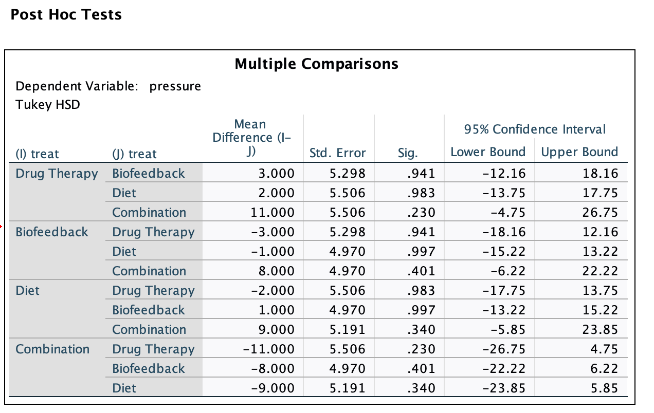
This output gives all possible pairwise mean comparisons in the treatment groups and does a Tukey QSD test for each. You can see in the left most column one group that is compared to a group in the second column. For example, the first row is the Drug Therapy group compared to the Biofeedback group. In this set up, there are some redundancies as each pairwise comparison will show up twice (the Drug Therapy vs Biofeedback comparison shows up again in fourth row for example). The significance column gives the p value based on the Tukey test, which you compare to .05, and the confidence intervals are already adjusted for the Tukey test.
Again, this isn’t the best example data set, but as we can see none of the pairwise comparisons are significant after controlling for experimentwise error rates using the Tukey test.
5. Scheffé’s Method
The Logic
Scheffé was designed for post hoc complex comparisons. This is the situation where you decide which contrasts to test only after examining the data, and your contrasts may include complex (non-pairwise) comparisons.
In this situation, Bonferroni should not be applied because \(C\) is not defined as you did not select a pre-specified set of contrasts. And Tukey does not apply to complex comparisons because Tukey only handles pairwise differences. Scheffé can be used when complex comparisons in both planned or post hoc comparisons. In planned complex comparisons, it competes with Bonferroni. In post hoc complex comparisons, it is the only option.
The key insight behind Scheffé is that, in a post hoc setting, you are implicitly searching across all possible contrasts. You are not just examining pairwise comparisons but any combination of group means. Among all possible contrasts, one of them will necessarily have the largest \(SS_\psi\) (the largest contrast sum of squares). Scheffé identifies what the maximum \(F\) statistic could be under this worst-case selection and uses that as the critical value. In this sense, it operates with a similar philosophy to Tukey’s HSD test, but it operates in a braoder spectrum of possible contrasts.
To get in the weeds a bit (the techncial details are not htat important), it turns out that the worst-case contrast can capture at most all of the between-groups sum of squares, \(SS_B\). Since the omnibus \(F\) statistic (the \(F\) statistic from the original ANOVA) is \(F_{omnibus} = SS_B / [(a-1) \cdot MS_W]\), the maximum possible contrast F is:
\[F_{max} = (a - 1) \cdot F_{omnibus}\]
This leads directly to Scheffé’s critical value, which is helpful to know:
\[CV_{Scheffé} = (a - 1) \cdot F_{.05;\; a-1,\; N-a}\]
This is a fixed value that depends only on the number of groups and the error degrees of freedom. It does not change regardless of how many contrasts you test. That is what makes Scheffé appropriate for post hoc work: you do not need to pre-specify \(C\).
Another conseqeunce of this is that the Scheffé test cannot be significant if the omnibus test is not significant. Therefore, it is not possible for you to get a Type I error for the Scheffé test being significant in scenarios where the main ANOVA is not significant (this is not true for Bonferroni or Tukey). It is also guaranteed that one Scheffé contrast test will be significant if the omnibus ANOVA was significant.
This isn’t that important in practical research, but at least can inform you if you did something wrong.
This formula for the CV will become important in the next section where we should compare the Scheffé to Bonferroni approaches. If you are interested in the \(F\) statistic or confidence interval equations for this method, I suggest you look them up. Note that they are different than the general formulas for the \(F\) statistic.
Before we move on, it is important to note that Scheffé requires equal variances. If heterogeneity of variance is present (aka, the group variances in their data is not equal amongst eachother), Scheffé is not appropriate.
Scheffé vs. Bonferroni: When to Use Which
As specified before, in situations where you are doing a post hoc comparisons of complex contrasts (i.e., non-pairwise contrasts), you must use Scheffé because Bonferroni requires planned comparison contrasts (\(C\)). However, in situations where you are looking at complex contrasts that were planned, then it is possible to use either Bonferroni or Scheffé.
In this scenario, the question is which one gives you more power (i.e., lower critical value) for your specific situation and which one is more conservative (i.e., lower Type I error but lower power). The answer depends on how many comparisons you are making:
| C (# Comparisons) | Bonferroni CV | Scheffé CV |
|---|---|---|
| 1 | 4.17 | 8.76 |
| 2 | 5.57 | 8.76 |
| 3 | 6.45 | 8.76 |
| 4 | 7.08 | 8.76 |
| … | … | 8.76 |
| 9 | 8.94 | 8.76 |
| 10 | 9.18 | 8.76 |
(For \(a = 4\) groups, \(df_{error} = 30\).)
Bonferroni’s critical value increases with \(C\), while Scheffé’s stays fixed regardless of the number of contrasts you are comparing. In this example, they cross over at around 8 comparisons. So, as a general rule:
- For a small number of planned comparisons, Bonferroni has more power and should be preferred.
- For a large number of comparisons or post hoc complex contrasts, Scheffé is preferred (and may be the only valid option).
- Scheffé should not be used unless at least one comparison is complex. For pairwise-only post hoc comparisons, use Tukey.
In terms of scenarios where you want to optimize your power, you will need to calculate the CV’s and go with the method that has the smaller value. You can use the same online calculator for Bonferroni as I gave above (repeated here for convenience):
Here’s a calculator I like. There are two caveats:
- You must make the first degree of freedom 1 and the second degree of freedom \(N-a\).
- You need to put in your adjusted alpha level \(\alpha /c\) in the probability level.
For Scheffé’s test, you can actually use the same \(F\) critical value calculator. There are a few important caveats though:
You will use the regular \(F\) statistic degrees of freedom. That is, the first degree of freedom is \(a-1\) and the second degree of freedom is \(N-a\).
The alpha level should stay at \(\alpha = .05\).
After you calculate the \(F\) statistic using the two above steps, you must multiple this \(F\) value by \((a-1)\). E.g., if you got an \(F\) value of \(3.2\) with \(a=4\) groups, the Scheffé critical \(F\) value is \((4-1)3.2 = 9.6\). This last step is important because if you do not multiply the \(F\) value you get from the calculator, your CV for the Scheffé test will be wrong.
The last thing is to compare the Bonferroni value and the Scheffé value and go with the test that has the lowest CV. Again, there is not an easier way of doing it. So if you are really worried in a case where you are doing planned comaprisons, you could always just do Bonferroni (as this is the most common and easily defended). Bonferroni will be more powerful if you don’t have a large number of groups (common in psychological researcher). Just note that you might be at more risk of Type I error if you don’t compare.
Scheffé in SPSS
To apply a Scheffé correction, you need to use MANOVA. (Note, I am aware of a few other options to get you “Scheffé” test results in SPSS, however I honestly don’t know what these are doing as the results are wrong. So just use this method.). First, change the /cinterval line to use the joint and univariate Scheffé specification:
MANOVA pressure BY treat (1 4)
/print=cellinfo(means)
/error=within
/cinterval = joint(.95) univariate(scheffe)
/contrast(treat) = special (1    1    1    1
                             1    1    1   -3
                             .5   .5  -.5  -.5
                             1   -1    0    0)
/design = treat.
Two things have changed from the Bonferroni syntax:
The /cinterval line now uses joint(.95) univariate(scheffe). joint(.95) keeps the family-wise error rate at .05 across all contrasts tested together. univariate(scheffe) specifies the Scheffé method for each individual contrast interval.
The /design line has changed from treat(1) treat(2) treat(3) to simply treat. This is critical. MANOVA uses the /design line not only to specify what goes in the model, but also to define what constitutes a family of tests (a family of tests simply means the set of comparisons over which the experimentwise error rate of .05 is being controlled together). If you leave it as treat(1) treat(2) treat(3), MANOVA treats each contrast as its own separate family, which sets \(\alpha_{PC} = .05\) for each one individually, defeating the purpose of the correction. Writing /design = treat. tells MANOVA to treat all contrasts together as a single family, so the correction applies across all of them jointly.
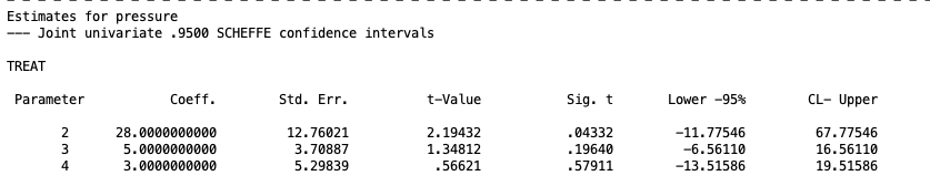
This output gives you the contrast \(\Psi\) coefficients, their standard errors, the \(t\) statistics (square them to get the Scheffé \(F\) statistics), and Scheffé 95% confidence intervals.
Critical warning about the Scheffé output: The \(p\) values in the Scheffé MANOVA output are not corrected. Do not use them for significance testing. SPSS provides the Scheffé-corrected confidence intervals and the \(t\) statistics, but the printed \(p\) values are the ordinary uncorrected ones. To assess significance with Scheffé, you must either:
- Compare the calculated \(F_\psi = t^2\) to the Scheffé critical value \((a-1) F_{.05;\; a-1,\; N-a}\), or
- Check whether the Scheffé confidence interval excludes zero.
This is just a limitation of SPSS.
For our hypertension example with \(a = 4\) groups and \(df_{error} = 16\) (since \(n = 5\) per group, \(N = 20\)), the Scheffé critical value is:
\[CV_{Scheffé} = (4-1) \times F_{.05;\; 3,\; 16} = 3 \times 3.24 = 9.72\]
Any contrast F statistic must exceed 9.72 to be declared significant. In our cases, none do, and we can also see how 0 is contained within each of the confidence intervals too.
7. Summary: Choosing Your MCP
The choice of correction method comes down to your research context. I recommend referencing the flow chart I gave above, but here are some rules of thumb.
| Situation | Recommended Procedure |
|---|---|
| Small set of planned contrasts (pairwise or complex) | Bonferroni |
| A larger set of planned pairwise contrasts | Comapre Bonferroni and Tukey CVs; use the lower one |
| All pairwise comparisons planned or post hoc | Tukey |
| Post hoc complex comparisons | Scheffé |
| Planned contrasts with many comparisons | Compare Bonferroni and Scheffé CVs; use the lower one |
A few additional reminders:
- Tukey and Scheffé require equal variances. If the homogeneity of variance assumption is violated, use Bonferroni (which can accommodate heterogeneous variances via the unequal variance formulas).
- Tukey cannot be implemented via MANOVA in SPSS; use
ONEWAYfor Tukey. - For Scheffé in MANOVA, always use
/design = GROUP_VARIABLE(not the individual contrast design) to ensure the correction applies family-wide. - For Scheffé, never use the output \(p\) values. Only use the \(F\) statistic vs. the critical value or the confidence intervals.
- If the omnibus ANOVA is non-significant, Scheffé will never find a significant contrast. You can skip it.
8. Bonus: False Discovery Rate
All of the procedures covered so far control the “familywise” error rate. Aka, the probability of making any false positive across your whole set of tests (the whole experiment is a “family” in our scenarios, but families can be more specific). This is a strict standard, and it gets harder to satisfy as the number of comparisons grows.
An alternative approach, common when researchers run a very large number of tests (common in fields like genomics, neuroimaging, or any study with dozens of comparisons), is to control the false discovery rate (FDR) instead. Rather than asking “what is the chance of even one false positive?”, FDR asks a more forgiving question: “of the tests I declare significant, what proportion are likely to be false positives?”
For example, controlling FDR at .05 means that, on average, no more than 5% of your significant results are expected to be false positives, not that there is only a 5% chance of any false positive occurring at all. This distinction makes FDR considerably less conservative than Bonferroni or Scheffé, which is exactly why it became popular in contexts where dozens or hundreds of tests are unavoidable and familywise correction would leave you with almost no power to detect anything.
Imagine if you did 100 tests on neuroimaging data (I’ve seen much higher). The Bonferroni corrected level would be \(.05/100 = .0005\), which is lower than many programs will even print for you by default. It’s just not practical. So the FDR method gives researchers a way to correct for error after they concluded significance on a regular \(\alpha=.05\).
The most common method for controlling FDR is the Benjamini-Hochberg procedure, which ranks your \(p\) values from smallest to largest and compares each one to a sliding threshold rather than a single fixed cutoff.
We will not cover the mechanics of FDR control in this course, since our designs typically involve a small, manageable number of planned or post hoc contrasts where familywise correction is appropriate. But it is worth knowing that FDR exists as the standard approach once the number of comparisons becomes very large, and you may encounter it when reading research in other fields.
Discussion Questions
Q1. Using the hypertension data, a researcher runs all 6 pairwise comparisons after looking at the data and seeing that groups 1 and 4 look particularly different. What should \(C\) be set to, and why? Which method would you recommend?
Q2. A researcher plans 3 contrasts before data collection: one complex and two pairwise. Which correction method(s) are appropriate? What would you need to compare to decide between them?
Q3. Explain in your own words why the \(p\) values in the MANOVA Scheffé output cannot be used for significance testing. What can you use instead?
Q4. Without using \(p\) values, how can you assess whether a contrast is significant? Use a worked example from the ONEWAY output above to illustrate.
Q5. Using the decision tree, classify each of the following scenarios and identify the appropriate MCP:
- 4 groups; all 6 pairwise comparisons; planned in advance.
- 4 groups; 3 planned complex contrasts.
- 4 groups; 2 pairwise and 1 complex; decided after looking at the data.
- 4 groups; all pairwise; decided after looking at the data.
Q6. Suppose you have 4 groups and \(df_{error} = 30\). You are planning 4 complex comparisons. Looking at the Bonferroni vs. Scheffé critical value table, which method should you choose? At what number of comparisons does your answer change?
Well Done!
You have completed the Multiple Comparisons lesson. Here is a summary of what was covered:
- How running multiple tests inflates the experimentwise Type I error rate
- The distinction between per-comparison and experimentwise error rates, and the formula \(\alpha_{EW} = 1 - (1 - \alpha)^C\)
- The difference between planned and post hoc comparisons, and why post hoc selection inflates \(C\)
- The three main correction procedures: Bonferroni (flexible, best for small planned sets), Tukey (best for all pairwise), and Scheffé (best for post hoc complex comparisons)
- How to implement each in SPSS using
ONEWAY(for Tukey and simple pairwise) andMANOVA(for Bonferroni with/cinterval=individual(#)and Scheffé with/cinterval=joint(.95) univariate(scheffe)) - The critical gotcha for Scheffé: never use the output \(p\) values; use the \(F\) statistic vs. the critical value or the confidence intervals
- The link between Scheffé and the omnibus F test